Credit Risk Modelling for MSMEs

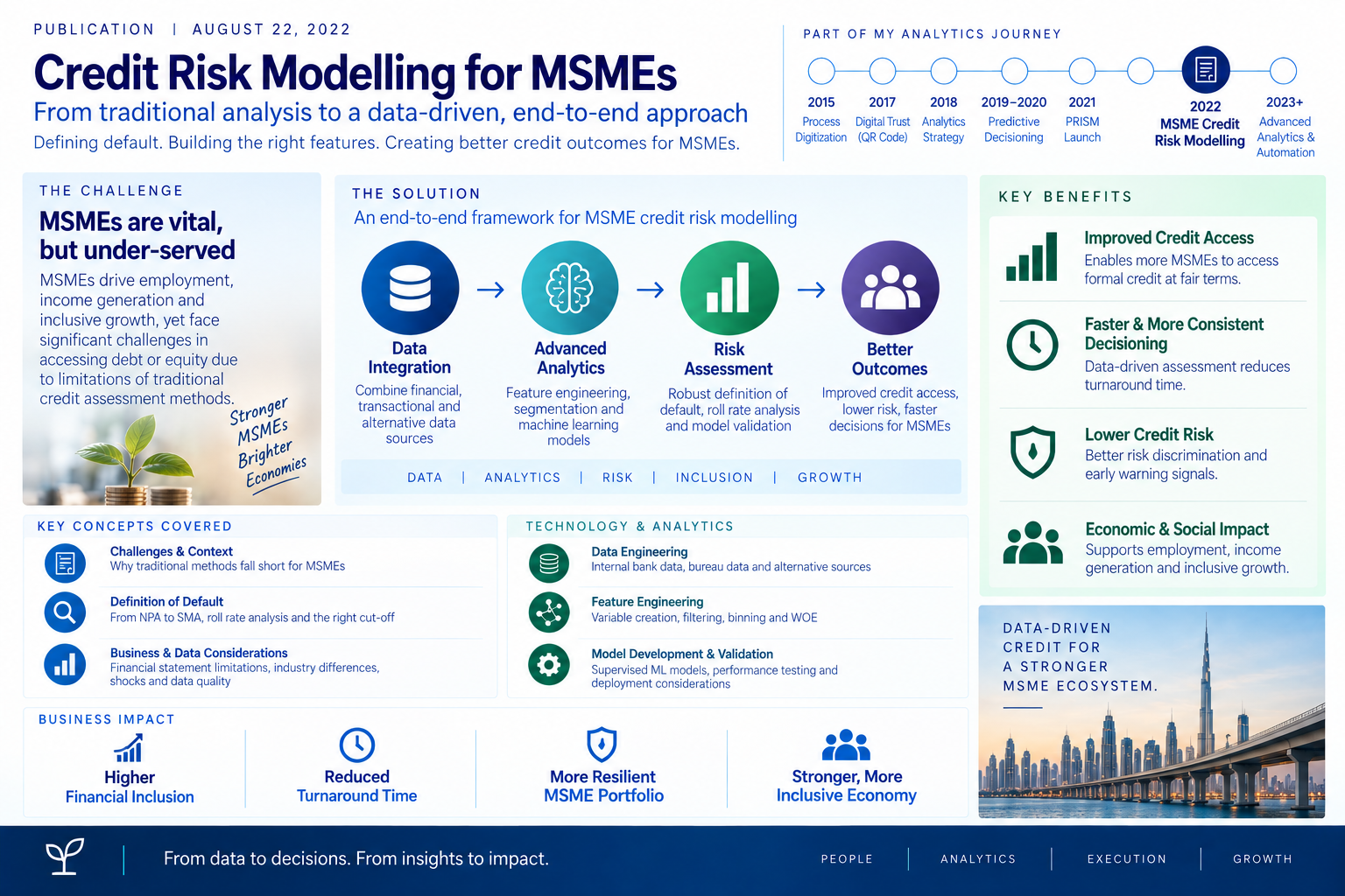
Small and Medium Enterprises play a vital role in the economy of a country. It is a well-documented fact that they contribute to income generation, employment creation and poverty alleviations. However, SMEs continue to struggle to raise capital in form of debt or equityⁱ. Part of the problem arises due to lack of efficient ways of credit risk assessment for MSMEs. Most of the conventional methods of credit risk assessment for enterprise borrowers have not been optimally designed for MSMEs. This series of articles will look at the ways of improving credit access for SMEs using business analytics and data science. Some of these ideas and solutions have been implemented at various banks and NBFCs and others are at an early stage of evolution.

Credit risk analysis – designed for corporate used for MSMEs

In the past years, the pre dominant method of credit analysis has been financial statement analysis. Majority of credit analysts have been trained on using financial statement analysis, there are well-defined rules and methodologies for using this type of analysis. The Reserve Bank of India keeps on publishing reports and norms from time to time. While financial statement (profit and loss account and balance sheet) analysis is a good starting point for credit assessment, and it works well for large corporate, it has various shortcomings that one realises if one tries to apply these methods and norms to Micro Small and Medium Enterprises (MSMEs). The major shortcomings are described below.

Lack of varied benchmark

The number of large corporate in India is much smaller compared to MSMEs. Given a small sample size, a certain level of homogeneity can be assumed for financial metrics for these companies. To give an example, one can say a current ratio of 1.33 is a satisfactory indicator of liquidity. In fact, it is this number, which has been treated as magic formula in various textbooks and RBI reportsⁱⁱ. However, the large MSME population is very varied and same benchmarks cannot be used for accurate credit assessment.

Less shock absorbing capacity

A large corporate is a like a strong adult who can with stand relatively bigger shocks. An MSME is a like young child who will find it more difficult to survive after a similar shock. In the recent past, we had few such system wide shocks in form of demonetization, GST implementation and Covid-19 induced lockdown. There are also idiosyncratic shocks that are specific to the individual enterprise. A few examples are – lack of sale for a few weeks, death of promoter, accidents in factory premises etc.

The issue with financial statements is that they are published with considerable time lag. Consider a hypothetical scenario that an MSME had a fire in its factory in the month of May. The implication of this event shall be recorded in some form in the Profit & Loss statement of the financial year in the year ending of March of next year. The Balance sheet shall be finalised in the month of October or November of the next year. Thus, it is likely that there is a gap of 17- 20 months between the actual occurrence of the event and communication of its impact to the lender. A large corporate would have managed to survive and recover in the interim due to its better resilience, but same can’t be said for an MSME.

Less reliable financial statements

The financial statements of MSMEs are not of the same quality as that or large corporate because many a time they do not have dedicated and skilled finance and accounting professionals on role. They cannot afford same quality of financial auditors as large corporate and compliance is a significant cost of business for a small sized firm. In addition, there is the common issue of adverse selection and lemons problemⁱⁱⁱ. Thus, due to a few unscrupulous borrowers, everyone is looked at with suspicion and denied credit at terms favourable to them.

Possible solution

Advanced analytics and data science offer solutions to these problems. With the increased availability of data capturing, storage and processing capabilities, these solutions can be used by a higher number of lenders. In the initial days of credit model development, the top users of these models were credit card and personal loan departments of banks. Over the past years MSME and business banking divisions are trying to catch up. The catch is that while the underlying algorithms and data science techniques used by business banking analytics are same as those used by retails banking, the type and nature of variables are very different. Therefore, there is a need of professionals who are skilled in the areas of corporate credit assessment, data science and business analytics to create models for business borrowers. MSME credit teams need to generate ideas, which are suitable for credit risk assessment of business loan and convert these ideas to robust credit risk assessment models.

Fortunately, due to advances made in data science, it is now possible to customize the financial analysis for MSME portfolios. In this section, I describe the first step for developing a probability of default (PD) model. In the subsequent sections, I will describe financial and other data sources that can be used for creating a PD model. Then, I will describe the logic of variable selection from these sources. That will be followed by the steps of feature engineering, feature selection and model development. The latter steps are common across models. Finally, I will demonstrate how an integrated model gives a comprehensive credit score for the MSME borrower with a high prediction power and accuracy. MSMEs.

How bad is really bad?

PD models fall in the category of supervised machine leaning. That means that the data scientist has to tell the machine that which are the borrowers, which actually defaulted, and which are those that did not. That brings us to the fundamental question of what is default.

The word default can mean various things to various people. In the world of external credit rating (think of Standard & Poor and Moody’s) a delay of one day in paying the instalment of a loan or the interest on it by even one rupee is a default. So if you do not want to be classified as a Default – pay all the money due on or before the due date. This is a very stringent definition and was designed for bond issuers. Bond markets operate differently than banks loans. In the bond market the investor does not have any direct contact with the issuer. He/ she has bought the bond based on independent credit risk assessment done by a rating agency. Therefore, slightest delay in repayment should alarm him/her. For more details on evolution and role of the external credit rating agencies, may refer to this excellent report by Dr Y V Reddy, Ex Governor of the Reserve Bank of India^iv

Evolution of definitions – NPA to SMA

Banks by contrast have a complete knowledge of the business of the borrower and their key stakeholders. While banks are also very stringent in the matters of non-payment of dues by a borrower, the impact of this is more pronounced when there is continuous delay of 90 or more days in the repayment by the borrower. In the banking industry, such accounts are called Non Performing Assets (NPA). And, NPA is a bad word for bankers. These are assets that banks hold but they do not generate any income and hence are non performing. The moment as asset is classified as NPA banks have to provision for loss.

In the year 2013 RBI came up with a discussion paper on ways to reduce stress in the banking system and early resolution of stressed accounts^v. They came up with new category called Special Mention Account (SMA). The idea of SMA had been discussed earlier in the year 2002 in another notification of RBI^vi. This concept was implemented in 2014 and created three categories of stressed account before it could be classified as NPA.

Approaching the problem statistically

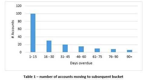
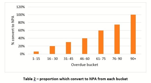
We perform a roll rate analysis to identify a good definition of default. Essentially, we look at all the cases which were in overdue category on a given date and observe how many of those correct themselves by repaying the money due to the bank, and how many deteriorate further in the next 5, 30, 45, 60 days and so on. That gives us a sense of when should an alarm be raised.

The graph below shows a hypothetical roll rate analysis.

Selecting a definition of default

In the above-mentioned hypothetical example, 60+ ever in the next 12 months seems to be a good cut off. By using this cut off, we are not acting too late and we know that if an account is predicted to default there is a 60% chance that it will actually do. At the same time, we are not classifying too many accounts as default and we manage to keep false positive rate low. It should be noted that different banks with different risk appetites, might be more conservative or liberal in the selection of default definition.

In case the borrower has loan above ₹ 5 Cr, the lending bank has to disclose its name to CRILC and mention the status – standard, SMA 0, SMA 1 etc. In such a scenario banks might want to change the definition of default to SMA 0 (one day delay in the payment of interest or principal). Because once the details are shared with RBI, it is known to all the banks in India and none of them might be willing to take over the account.

It also depends on the business segment. Few business segments, which charge higher interest rate and generate more business volume can be more liberal and vice versa. Thus, selection of default definition is a very important decision and should be made in discussion with team members of business (sales) and credit functions after performing the roll rate analysis as described above.

In the previous section, I discussed the definition of default. In this section, I will try to throw some light on a few other important concepts of credit risk modelling.

Standard process of predictive modelling

The standard process for developing a predictive model is as follows:

a)      Identify the target/ dependent variable

b)     Identify the independent variables

c)      Use data science algorithms to establish a relationship between the two

d)     Test the relationship/ rules so created on a different sample

If you want to know about these steps in more details, you may refer to a very good content created by MIT^vii . I will proceed to describing the process of selection of these variables for business borrowers. It is my endeavour to explain the process one-step at a time and focus more on the rationale behind it.

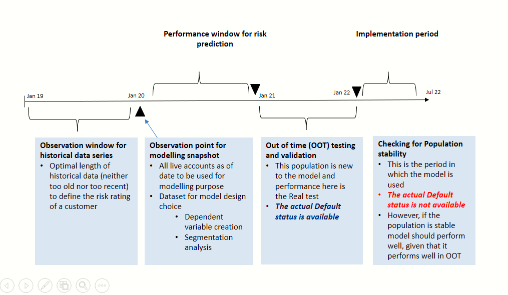
Observation point

It is the point in time when the model would be used to score the borrower. Alternatively, in the traditional manner, the under writer would perform the credit assessment.

Observation window

We want to know the characteristics or features of the borrower at the time of credit assessment (under writing). These characteristics are referred to as independent variables in the language of data science. The key questions to be answered are:

a)      What information is available to us?

b)     How old is the information?

The answers to these questions have a major bearing on the outcome. If the information is from a limited number of sources, then the model might not be comprehensive. On the other hand, if we want to include more sources of data we might have to look at a longer period for observation window.

The major sources of information are the financial statements of the borrower and data on its banking behavior, which is, captured in its Bank Statement and Credit Bureau (Think CIBIL, Equifax etc.) records.

MSMEs publish their financials once in a year; credit bureau records are update every month and bank statement is updated every day. Thus, if we choose 12 months of period in past then we would be able to balance comprehensiveness and recency of data. At the stage of feature selection, we may choose how many months of performance to look at for the data sources, which are updated more frequently. I will discuss this in detail when I write about the feature engineering part.

Performance window

At the time of credit assessment, we want to predict the performance of the account for some time in future. The appropriate time may vary with the size of the borrower, the type of loan facility and the bank’s ability to make a timely exit from the account. Other factors that influence this decision are the collateral^viii cover and legal environment, which enables banks to liquidate the borrowers’ assets and get their pound of flesh.

Long-term rating / through the cycle PD – It refers to a credit risk for a few years – usually 5 to 10 years. This is relevant if the bank is funding a project of the borrower, which might lead to cash generation after a few years, and hence bank needs to assess the credit for a longer period in future.

Short-term rating / point in time PD – it refers to credit risk arising out of financing for short term. It is usually taken as loan for up to one year. Borrowers use this money for meeting their working capital requirements.

In our hypothetical model, the performance window is one year because we want to use it for under writing of short term loans and would recommend a comprehensive assessment again after a year using updated financial statements.

Out of Time Testing

Once the sample data has been obtained for model development, it is divided in two parts – training set and testing set. We use training set data to develop the model and it is then tested on testing set data. It is imperative that the model is able to predict better than the current method of credit assessment, and whether it is approved or discarded depend on the results of testing.

However, we must keep in mind, that the basic premise of model development is that all the factors other than the ones being considered are same for the population on which the model is being run and the one on which it has been developed (ceteris paribus).

This assumption might not hold true in two different periods. There are many economic factors, which may affect the credit worthiness of the borrower but are not captured in the data used for model development.

If we are able to test the performance of the model in a different time and it delivers a good result that increases the confidence in it.

Implementation period

If a model passes the tests I have briefly described, it can be put to use. We refer to that as deployment. The period of time in which the model is actually used is called the implementation period. Once the model has been put to use, it should be periodically tested if it continues to work well or does it need to be modified. The way to monitor is check the stability of the population on which it is being used.

The fundamental difference between the previous two periods (performance window and out of time testing) and the implementation period is that the actual performance of the borrower is not known in this time. The user has to wait up to 12 months to see whether the borrower defaulted or not.

Coming full circle

Now, that I have described all the major time period and default definition, I want to draw your attention to the concept of population stability and why it is important in selection of the various time periods described so far. Model is essentially a rule to separate potential good borrowers from potential bad borrowers when none of them have actually defaulted. It is a very important point. The prediction is made on the basis of other known characteristics of the borrowers referred to as independent variables. The fundamental assumption here is that the unknown characteristics of the borrowers are same and the populations is otherwise stable (except for the independent variables considered for model development)

If the two populations are not similar in the aspects described above, then the rules / model may not work. To drive home my point, I will use an example from more common and natural comparisons.

Selecting soldiers

All countries have put in place rules on the physical traits of people interested in joining the armed forces. For India, this rule is a minimum height of 165 cms. This rule is believed to be effective in separating potential good soldiers from not so good soldiers. Imagine that the same rule was applied in Denmark. The average height of a Danish man is 181.38cm^ix. This rule would clearly not work because the underlying population is dissimilar and almost everyone would pass the test.

This was a very simplistic example. I will discuss examples pertaining to finance at the time of development of models and selection of independent variables.

How to select good observation window

Now we know that stability of population is a very important condition for the model to perform well. It implies that we should be careful in choosing the right period for the observation and performance window. The thumb rule is that one should choose a period of relatively less turbulence in the economy. I emphasize the word relative because there is always some or other shift taking place in an economy.

It is easier to understand this with a recent example. In the wake of Covid 19, governed of India implemented a lock – down in the country. This was followed by Reserve Bank of India commanding the banks to impose a moratorium on all the borrowers for 3 months (this was later extended by another 3 months for few subsectors^x). This moratorium started from 1st March 2020. Under the conditions of the RBI notification, all the accounts that were standard at the beginning of the moratorium were to be considered so for the next 3 months.

The consequence of this rule was that there would be over dues for enterprises, that were experiencing some kind of financial stress before march 1st 2020 as well as those that were not. In other words the independent variables would not be able to separate potential good borrowers from the potential bad borrowers.

I have described a few core concepts of the process of credit risk model development. In the next section I will move to details of financial model’s variable selection.

In section 1, I discussed what are the short comings of financial statements when it comes to credit assessment of MSMEs. In this article I will try to explain the meaning of financial variables / features and how do one can drive some inference about the loan repayment ability of a borrower. Same features will be used later to create a credit risk assessment model for MSMEs.

Financial statements – content and meaning

Every business works with the objective to make money and therefore they record their activities in the terms of money. There are two statements all the businesses produce periodically – Profit & Loss/ Income Statement and Balance Sheet. The income statement gives information about the sales or income and costs of the business during a time period. Both sales and costs can be further subdivided in sub headings. The balance sheet tells the reader about the assets and liabilities of a business on a given date.

Banks want to give money only to those individuals and enterprises who are likely to return that money and usually along with some interest. Thus, bankers pay a close attention to these two statements. I will now go on to delve in some more details in the individual components of these two statements and variables that can be created from these.

Those of you who want to understand financial statement analysis can refer to an excellent book by Ciby Joseph^xi. Since this article is written for people interested in credit modelling, I will keep focus on that and mention the tools of financial analysis very briefly. My objective is to help the reader understand the logic behind the financial statement and create features for their model. Those who want to learn conventional way of financial statement analysis can refer to the aforementioned book and others books written on the topic.

Income statement

A few variables categories which can be derived just from income statement are: total income, income from operations, fixed cost, variable cost, profitability etc. each of these categories tell us a story about the status of the enterprise and can help building the credit risk model.

Income and expense

If a business is running well, it should generate consistent sales and the sales should also grow with each year. Otherwise, questions arise about the demand of the enterprise’s product or services and their ability to serve existing and/or new customers.

However, the income by itself does not tell much. In the world of credit modelling, it is called a raw variable. It is better to create a new variable by comparing it with something else. First step is to look at income from operations. It tells us if the business is able to make money from its main economic activity. It can also make money by selling some assets. But that income is not going to be regular and does not indicate healthy business.

Change in income

Our country has a relatively high growth rate when compared to other countries. The GDP growth rate for us is usually in the range of 6-8% per annum and that is in real terms^xii. That means if we add the price rise of 5- 7% per annum the growth rate is 11 – 15%. A healthy business is expected to increase its sales year on year (except in cases where the last year had some exceptional income).

Profitability ratios

Profit is not a dirty word. All businesses need to make profit to stay afloat. If a business does not make profit, eventually, that will lead to depletion of capital and it will shut down. Profit is realized when the sales is more than the cost, or, in other words, income is more than expenses. But expenses are of various kinds and are accounted for in a certain order.

Gross profit margin

In simple terms this is the sales minus the cost of goods sold. These are the direct costs and are mostly variable. Every business can choose how much raw material they want to buy, convert it to finished goods and sell those. It can also be called Earnings Before Interest Taxes Depreciation and Amortization (EBITDA). As a rule, businesses are supposed to pay their creditors (banks/ NBFCs) before they pay tax to the government. Depreciation and Amortization are not actual cash expenses but are merely apportioning of money already spent. However, they are important as an indicator of time after which the assets might have to be replaced. It is an important variable as it tells us whether the business has enough money left after the operations to pay for the fixed costs.

Net profit margin

After paying the variable costs, the business also has to pat costs which are more fixed in nature like salaries, rent etc. While nothing is permanent, these are cost heads which are difficult to reduce frequently. It is very difficult to fire employees or change the location of factory/ office every quarter or every year. By contract if business can use the raw material procured in the last quarter in the current quarter (provided it is not perishable).

Benchmarking kicks in

I will request the user to take a pause at this juncture. We discussed that it is not the income or the profit as such which matter, but the profit at the percentage of income. Now, I take the argument one step ahead and illustrate that it is not the change margins as such which matter, but how does it compare to other players in the same industry, region etc. We will discuss more of this in the section on benchmarking and we will keep on revisiting this line of argument.

In an industry and region which is very competitive, the profit margins shall be low. If the price of raw materials increases and the manufacturer is not able to pass on the increase to its customers, then the gross profit margin will go down (we saw this in case of industries using sunflower oil in the aftermath of Russia Ukraine war). But it is possible that there were other businesses in the same industry and region who were able to increase the price of finished goods. Thus, their gross profit margin did not dip as much as others.

Same rule applies to net profit where one enterprise had lower rent, or better technology leading to electricity cost.

Balance sheet

A few variable categories which can be derived from balance sheet are: liquidity ratios like current ration, quick ratio, leverage ratios like debt-to-equity ratio, fixed assets to adjusted tangible net worth (ATNW).

Assets and liabilities

All operating business have assets and liabilities. Asset is something which generates cash and liability is something which consumes or reduces cash. Plant and machinery for a manufacturing set up is an asset because it helps the business produce goods that can be sold for money. Similarly, inventory is an asset for a trader who can sell it and generate cash. Assets are always equal to liabilities.

When payment is due to some other party that is treated as liability. If a business has bought goods or services from another business then that amount is a liability. If they have not paid salaries to employees or rent to the landlord then those are liabilities. A going concern is supposed to honor their liabilities and the counterparties can go to court in case of any grievance related to non-payment. Liabilities are always equal to assets.

Long term and short-term assets and liabilities

If a business wants to create an asset it needs money for it. An asset can be a long term assets like machinery, patent, brand etc. which shall continue to generate money for years. Or it can be short term which has to be converted to cash quickly like inventory of finished goods, debtors (other businesses which owe you money because they bought something from you.)

Similarly, the liabilities can also be long term which you need to repay over years or short term which you need to repay in a few days, months or weeks. Examples of short-term liabilities are operational creditors, banks, provision for taxation, provision for leave encashment etc.

One important question is who are people who have given you capital for long term and what are their expectations vis a vis people who have given capital for short term and who gets precedence over whom.

Providers of long-term capital

Equity: The promoters of a business bring their money to start business and get money from friends and family. This is more common in case of MSMEs who do not have access to formal capital. These people have more faith in the entrepreneur and they believe that the business will generate enough cash over the years to pay them dividend (for equity holders) and repay the loan with interest (banks). They are not in a hurry to get their entire money back immediately and realise that there can be times when they are not paid and have asked for a higher share (return) for the risk they have taken.

In case of MSMEs their contribution appears as borrowing from subsidiaries or promoters’ relatives. Many a time it is shown as debt for tax purposes but in effect it is equity and should be considered as quasi- equity.

Providers of short- term capital

On the other hand, there are individuals and businesses who are willing to provide capital only for a short duration of a few days/ weeks/ months. They trust the enterprise that it will be able to create and sell product or services from the inputs they have provided in the terms of credit and repay them at the end of days/ weeks/ months.

Businesses are supposed to first pay their trade counter parties, then the bank, then the income tax and finally dividend to the equity holders. Thus, equity holders have higher financial risk and expect a higher return. Banks who provide loan for long term (more than a year) also face a higher risk and expect a higher interest rate.

Liquidity ratios

This category of if variables indicate the ability of the business to meet its short-term obligations by liquidating (converting to cash) their short-term assets. We can look at some common liquidity ratios below.

Current ratio

It is the ratio of total current assets to total current liabilities.

Note – this list is not exhaustive.

Key thing to note is that the current assets can be sold (inventory) or converted to cash (receivables) relatively quicky. The business may offer discounts to its customers to get payment in lesser time and honor its short-term obligations.

Quick ratio

This change from current ration eliminates any assets which might take time to be liquidates are removed and gives the liquidity position in a more conservative scenario. Lenders for short term should be concerned about the liquidity position of the borrower and therefore liquidity ratios are very important to create a credit risk model for working capital finance.

Leverage ratios

Leverage ratios tell us about the capital structure of a business. We have seen that there are two sources of capital – debt and equity. If a business is such that its income id stable and fixed in nature then it can afford to have expenses which are fixed in nature. The cash generated by the sales can be used to pay the expenses generated during the operations. Debt is also a source of cost and it is fixed. Imagine a business such as toll road operator. In normal circumstances, the traffic on road does not reduce or vary much and such a business owner can afford to take higher loan which they can repay by the relatively stable cash flows. But, in businesses which do not expect steady cash flows (like fashion accessories) it can be very risky move to create fixed obligations in form of interest. We will see in the following articles that bench marking is very important for arriving the correct conclusion.

TOL/ ATNW

Total outside liability (TOL) as a proportion of adjusted tangible net worth (ATNW) is a very important leverage ratio for MSMEs. Many a time MSMEs borrow and lend to related parties and loans can be confused with equity share.

The higher the leverage the riskier is the obligor for the bank because their ability to generate cash which is free to be given to promoter is curtailed (free cash flow) and that makes the business unviable in the log run.

Turnover ratios

These ratios tell us about the ability of business to convert current assets and fixed assets to cash. The underlying principle is that a good business is one that is able to generate more cash from its assets and is able to do that fast. Thereby, the assets are more productive.

Fixed asset turnover ratio

Imagine a factory that uses very sophisticated (and costly) machinery but operates only 6 hours a day. The value of goods produced is much lower than the potential it has and it can be said that its capacity utilization is sub optimum. In simple term, they are not operating well.

Interpretation – higher ratio means that the unit is able to generate more sales from its fixed assets and is thus performing efficiently. One has to be, however, slightly cautious because a very high fixed asset turnover ratio may also mean that the assets are being over used and this can lead to potential disruption of operations in near future. A wise thing to do is to compare the ratio with peers. We will discuss the interpretation of the value at the stage of model development.

Many people also use the inverse formula of average fixed assets by sales. That is also correct and only the interpretation is reverse.

Inventory turnover ratio

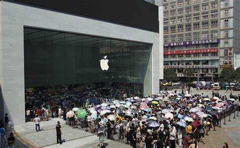
It answers the question – how fast is the business able to convert inventory of finished goods (or total inventory) to sales (the sale may be on credit leading to sundry debtors). A business which does so quickly saves on cost, enjoys a high demand for its products and should be able to make good profits. Imagine standing in que to buy an apple phone^xiii.

There can be various sub classifications of this formula that consider the inventory or only raw material (and this use cost of goods sold to calculate the ratio) or the work in progress inventory.

Another variable that can be created is inventory turnover in days. That is easier to interpret and tells that how many days does it take on an average to convert inventory to sales. Or, the inventory we are holding it equivalent to how many days of sales.

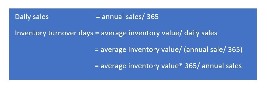
Interpretation

Inventory turnover ratio – higher the ratio, better it is. This should be taken for a normal business operation and not distress sales.

Inventory turnover days – the lower the better.

Debtor turnover days

In the traditional manufacturing businesses or product sales, there is a lag between the day goods are sold and the day payment is received. This is so because the buyer wants a few days’ time to inspect the goods and then it passes through the steps of payment. The days might vary depending on who the buyer is. I recall that when I used to work for Indian railways, there were as many as twelve steps between the receipt of goods and issue of payment cheque!

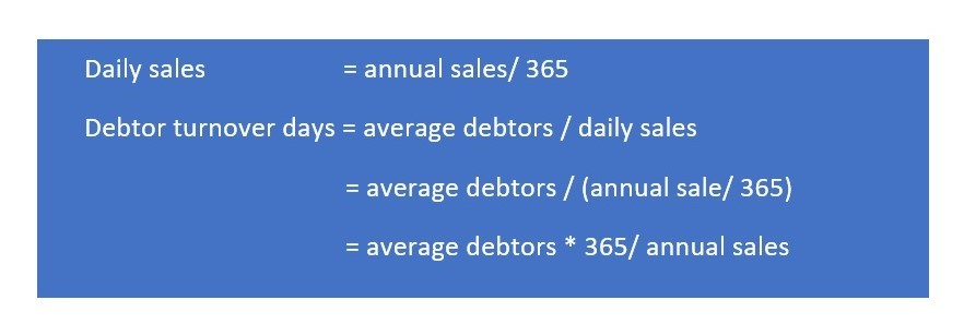
Interpretation

Banks would want to finance a business that is able to collect payment as quickly as possible. Thus lower the debtor turnover days, the better it is considered.

Summary of key ratios

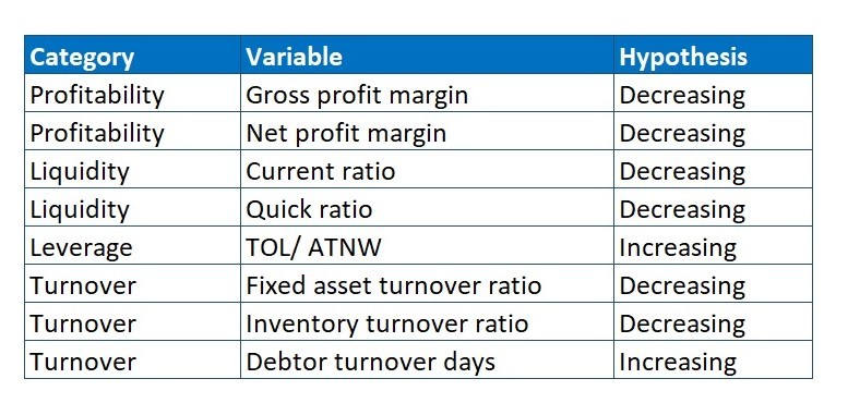
The table below shows the summary of all the ratios described in this article and the previous one. The last column shows the hypothesis of probability of default. Increasing means that a higher value of the variable should lead to a higher PD and decreasing means that a lower value of the variable should lead to a higher PD.

Monotonicity

A credit assessment model developed using logistic regression requires that there should be a high linear correlation between the default rate and value of the independent variable. It is referred to as monotonicity. This may not always be true in real life and in such scenarios, one should explore machine learning algorithms such as decision tree and random forest.

Next steps

I have completed the description of a few sample variables and the underlying logic for using those for financial analysis and development of credit assessment model. In the next section, I will explain the process of feature engineering and feature selection.

In the last section we saw the various types of financial variables which are used to assess credit risk. In the past few years, technology has evolved and better computing power allows us to try out more combinations of variables before we finalize the ones which we would want to use in a probability of default model. The process of creating variables and shortlisting the useful ones is called feature engineering (the independent variables being referred to as the features). In this article we will use the word feature and variable interchangeably.

Feature creation

As we have seen various variables like Gross profit margin, Fixed asset turnover ratio, Inventory turnover ratio etc. can be used to analyze credit worthiness of a borrower. We go one step ahead and create more features (variables) from these. This step requires imagination on the part of model developer. He/she has to imagine the features which should have an effect on the outcome. Like calculating the current ratio this year by the current ratio of last year thereby checking if the liquidity profile of the borrower has improved or deteriorated. I have listed a few features below. This list is not exhaustive as the purpose is to illustrate the process.

a.      Cash and bank balance/ Adjusted tangible net worth

b.      Cash and bank balance/ Net sales

c.      Total outside liabilities / Total assets

Going like this we can create 300 – 500 features from financial statements.

Feature selection

The next step is to reduce the number of features by selecting a few and rejecting others. Feature selection should be stepwise process allowing the model developer to analyze and evaluate features gradually.

Step 1 – Fill Rate & Univariate Gini

In this step we use two criteria to short list features – fill rate and univariate Gini. These are the simplest ways to identify features.

Fill rate

The first filter is fill- rate. We want to keep only those features which are available for a sufficiently large proportion of the population. If a variable is a great predictor of default, however, it is not available for many of the candidates then it is of little use. We measure fill rate as a percentage of records for which the variable is available out of total records. We reject all such variables which have a fill rate below a threshold. Selecting a threshold is call of the model developer. We have taken a fill rate of 90% for the feature to be retained.

Univariate Gini

Gini is a measure of predictive power of a model^xiv. Univariate Gini tells us how good a variable is in predicting the default all by itself. A good cut off can be 10% or 20% depending on the number of features created. One may use packages or libraries in R/ Python to calculate Gini.

Step 2 – Principal Component Analysis

In the next step we conduct Principal Component Analysis (PCA) to identify features which might have a bearing on the dependent variable.

Principal Component Analysis

Principal component analysis, or PCA, is a statistical procedure that allows you to summarize the information content in large data tables by means of a smaller set of “summary indices” that can be more easily visualized and analyzed^xv. PCA arranges the existing features in groups. Group 1 should have highest number of features and it indicates that those features are better predictors of default. Group 2 has fewer features and so on. We should select features in a way that we get maximum from top numbered groupings and also get features from various categories (turnover, profitability etc. – please refer to the previous articles).

Step 3 – Binning and Variable Transformation

In this step we perform two exercises. We bin the variables thus creating categorical variables from numerical and we transform the variables to be used for modelling.

Binning

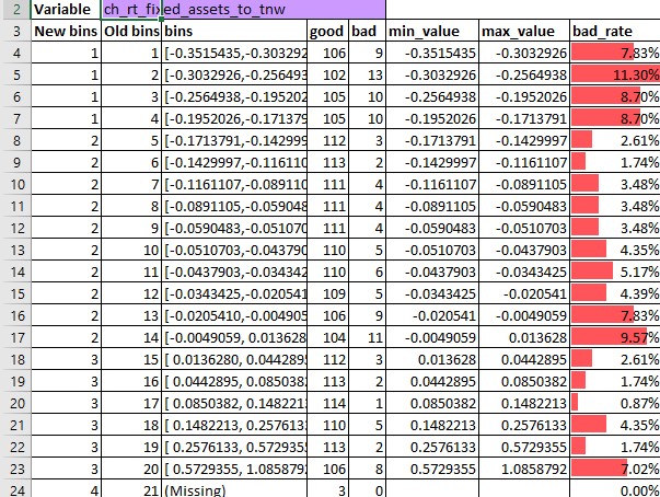
We put the variables in bins or class intervals and observe the “bad – rate” in those bins. Now for a moment let us take a diversion and use a different analogy to understand the importance of binning. Imagine that there are two kids of age five years and four years and you are asked if you think they are significantly different in their ability to talk and communicate. Your answer will most likely be no. But, if there are two kids with ages three and two and you are asked the same question, your answer might change.

When it comes to behavior the absolute difference in value might not matter as much as the threshold. And that is what binning does. Whether the interest coverage ratio of a company is 1.2 or 1.3 might not be very significant information, but whether it is 1 or 0.9 might create a lot of difference in its credit worthiness.

We bin the variables based on the bad rates in those bins. We start with 20 bins and gradually merge those till we get monotonicity in the bad rate. Please see the images below.

Variables Transformation

Earlier in this article, I have argued that we should use derived variables instead of raw variables for model development. The simple logic being that it does not matter how much current assets you have, what matter is what is the proportion of current assets to current liabilities. And then I extended that argument for creation of chaid variables. I take that argument one step ahead and say that what matter for a feature to be useful is the sample of “bads” contained in the bin divided by the sample of “goods”. We refer to this variable as Weight of Evidence (WOE) and use it for the model development.

Model development

The new variables thus developed can be used as independent variables in a logistic regression model. It is a very standard process and therefore I will not describe that in detail here.

References

- iCredit and Finance for MSMEs: According to the June 2019 report by the UK Sinha Committee constituted by the Reserve Bank of India (RBI), the overall credit gap in the MSME sector is estimated to be Rs 20-25 trillion (Rs 20-25 lakh crore)
- iiA borrowing unit will be required to contribute a minimum of 25 per cent of the total Current Assets out of its long term funds. This method of assessing MPBF known as the second method of lending, will, therefore, ensure a minimum Current Ratio of-I.33:1.Report of the committee to examine the adequacy of institutional credit to the SSI sector & related aspects 1992
- iiiThe lemon theory posits that in the used car market, the seller has more information regarding the true value of the vehicle than the buyer. This results in the buyer not wanting to pay more than the average price of the car, even if it is of premium quality. This benefits the seller if the car is a lemon but is a disadvantage if the car is of good quality.
- ivhttps://rbidocs.rbi.org.in/rdocs/Bulletin/PDFs/13292.pdf
- vhttps://www.rbi.org.in/scripts/PublicationReportDetails.aspx?UrlPage=&ID=715
- vihttps://www.rbi.org.in/scripts/NotificationUser.aspx?Id=899&Mode=
- viihttps://learning.edx.org/course/course-v1:MITx+15.071x+2T2020/block-v1:MITx+15.071x+2T2020+type@sequential+block@fbc8e7be7caf4032be2a0ece8a734586/block-v1:MITx+15.071x+2T2020+type@vertical+block@5a9af0d8ebf348889954f4dd4c68833e
- viiiPrimary security is provided when banks create a charge (claim) on the asset created out of the loan given. Collateral security is what they want by way of charge on other assets of the borrower (land, building etc.)
- ixhttps://www.insider.com/tallest-people-world-countries-ranked-2019-6#:~:text=Denmark%20%E2%80%94%20174.29cm%20(5%20feet%208.61%20inches)&text=The%20average%20Dane%20is%20174.29,5%20feet%205.83%20inches)%20tall.
- xhttps://www.rbi.org.in/Scripts/NotificationUser.aspx?Id=11835
- xihttps://onlinelibrary.wiley.com/doi/book/10.1002/9781118604878
- xiihttps://www.wallstreetmojo.com/nominal-gdp-vs-real-gdp/
- xiiihttps://metro.co.uk/2014/07/29/thousands-queue-to-enter-new-apple-store-in-china-4813411/
- xivhttps://www.crisil.com/content/dam/crisil/our-analysis/publications/default-study/crisil-ratings-annual-default-and-ratings-transition-study-fy-2022.pdf
- xvhttps://www.sartorius.com/en/knowledge/science-snippets/what-is-principal-component-analysis-pca-and-how-it-is-used-507186